Statistics and Probability
Welcome to Our Site
I greet you this day,
For the Classic ACT exam:
The ACT Mathematics test is a timed exam...60 questions in 60 minutes
This implies that you have to solve each question in one minute.
Each of the first 20 questions (less challenging) will typically take less than a minute a solve.
Each of the next 20 questions (medium challenging) may take about a minute to solve.
Each of the last 20 questions (more challenging) may take more than a minute to solve.
The goal is to maximize your time.
You use the time saved on the questions you solve in less than a minute to solve questions that will take more
than a minute.
So, you should try to solve each question correctly and timely.
So, it is not just solving a question correctly, but solving it correctly on time.
Please ensure you attempt all ACT questions.
There is no negative penalty for a wrong answer.
Also: please note that unless specified otherwise, geometric figures are drawn to scale. So, you can figure out
the correct answer by eliminating the incorrect options.
Other suggestions are listed in the solutions/explanations as applicable.
These are the solutions to the ACT past questions on the topics: Statistics and Probability.
When applicable, the TI-84 Plus CE calculator (also applicable to TI-84 Plus calculator) solutions are provided
for some questions.
The link to the video solutions will be provided for you. Please
subscribe to the YouTube channel to be notified of upcoming livestreams. You are welcome to ask questions during
the video livestreams.
If you find these resources valuable and if any of these resources were helpful in your passing the
Mathematics test of the ACT, please consider making a donation:
Cash App: $ExamsSuccess or
cash.app/ExamsSuccess
PayPal: @ExamsSuccess or
PayPal.me/ExamsSuccess
Google charges me for the hosting of this website and my other
educational websites. It does not host any of the websites for free.
Besides, I spend a lot of time to type the questions and the solutions well.
As you probably know, I provide clear explanations on the solutions.
Your donation is appreciated.
Comments, ideas, areas of improvement, questions, and constructive
criticisms are welcome.
Feel free to contact me. Please be positive in your message.
I wish you the best.
Thank you.
-
Symbols and Meanings
- $X$ = dataset $X$
- $x = x-values$ OR data values
- $x_{mid}$ = class midpoint of $x-values$ = class midpoint of the data values
- $\Sigma$ (pronounced as uppercase Sigma) = $summation$
- $\Sigma x$ = summation of the $x-values$
- $f = frequency$
- $F = frequency$
- $\Sigma f$ = summation of the frequencies
- $\Sigma fx$ = summation of the product of the $x-values$ and their corresponding frequencies
- $(\Sigma x)^2$ = square of the summation of the $x-values$
- $\Sigma x^2$ = summation of the squared of the $x-values$
- $\bar{x}$ is sample mean of the $x-values$
- $\mu$ = population mean
- $n$ = sample size
- $N$ = population size
- $\tilde{x}$ = median
- $\widehat{x}$ = mode
- $AM$ = assumed mean
- $D$ = deviation from the assumed mean
- $x_{MR}$ = midrange
- $LCL$ = lower class limit
- $UCL$ = upper class limit
- $min$ = minimum data value
- $max$ = maximum data value
- $LCB_{med}$ = lower class boundary of the median class
- $CW$ = class width
- $f_{med}$ = frequency of the median class
- $CF_{bmed}$ = cumulative frequency of the class before the median class
- $LCB_{mod}$ = lower class boundary of the modal class
- $f_{mod}$ = frequency of the modal class
- $f_{bmod}$ = frequency of the class before the modal class
- $f_{amod}$ = frequency of the class after the modal class
- $R$ = range
- $s$ = sample standard deviation
- $s^2$ = sample variance
- $\sigma$ = population standard deviation
- $\sigma^2$ = population variance
- $CV$ = coefficient of variation
- $z = z-score$
- $Q_1$ = lower quartile or first quartile
- $P_{25}$ = 25th percentile or first quartile
- $Q_2$ = middle quartile or second quartile or median
- $P_{50}$ = 50th percentile or median
- $Q_3$ = upper quartile or third quartile
- $P_{75}$ = 75th percentile or third quartile
- $IQR$ = interquartile range
- $SIQR$ = semi-interquartile range
- $MQ$ = midquartile
- $LF$ = lower fence
- $UF$ = upper fence
- $TM$ = trimmed mean
- $\Pi$ (pronounced as uppercase Pi) = $product$
- $\Pi x$ = product of the $x-values$
- $GM$ = geometric mean
Grouped Data
$
\underline{\text{Class Size or Class Width}} \\[3ex]
(1.)\;\; Class\:\:Width = \dfrac{Maximum - Minimum}{Number\:\:of\:\:classes} \\[5ex]
(2.)\;\; Class\:\:Width = LCI\:\:of\:\:2nd\:\:Class - LCI\:\:of\:\:1st\:\:Class \\[3ex]
(3.)\;\; Class\:\:Width = UCI\:\:of\:\:2nd\:\:Class - UCI\:\:of\:\:1st\:\:Class \\[3ex]
(4.)\;\; Class\:\:Width = UCB\:\:of\:\:a\:\:class - LCB\:\:of\:\:the\:\:same\:\:class \\[3ex]
(5.)\;\; Class\:\:Width = LCB\:\:of\:\:a\:\:Class - LCB\:\:of\:\:previous\:\:class \\[5ex]
\underline{\text{Frequency Density}} \\[3ex]
(6.)\;\; \text{Frequency Density} = \dfrac{\text{Frequency}}{\text{Class Width}} \\[7ex]
\underline{\text{Class Midpoints or Class Marks}} \\[3ex]
(7.)\;\; Class\:\:Width = LCB\:\:of\:\:a\:\:Class - LCB\:\:of\:\:previous\:\:class \\[5ex]
\underline{\text{Class Boundaries}} \\[3ex]
(8.)\;\; Lower\:\:Class\:\:Boundary\:\:of\:\:a\:\:class = \dfrac{LCI\:\:of\:\:that\:\:class +
UCI\:\:of\:\:previous/preceding\:\:class}{2} \\[5ex]
(9.)\;\; Upper\:\:Class\:\:Boundary\:\:of\:\:a\:\:class = \dfrac{UCI\:\:of\:\:that\:\:class +
LCI\:\:of\:\:next/succeeding\:\:class}{2} \\[5ex]
$
(10.) Shortcut for Class Boundaries
If the class intervals are integers:
Lower Class Boundary = Lower Class Interval − 0.5
Upper Class Boundary = Upper Class Interval + 0.5
If the class intervals are decimals in one decimal place:
Lower Class Boundary = Lower Class Interval − 0.05
Upper Class Boundary = Upper Class Interval + 0.05
If the class intervals are decimals in two decimal places:
Lower Class Boundary = Lower Class Interval − 0.005
Upper Class Boundary = Upper Class Interval + 0.005
...and so on and so forth.
$
\underline{\text{Relative Frequency}} \\[3ex]
(11.)\;\; RF\:\:of\:\:a\:\:class = \dfrac{Frequency\:\:of\:\:that\:\:class}{\Sigma Frequency} \\[7ex]
\underline{\text{Cumulative Frequency}} \\[3ex]
(12.)\;\; CF\:\:of\:\:1st\:\:Class = Frequency\:\:of\:\:1st\:\:Class \\[3ex]
CF\:\:of\:\:2nd\:\:Class = Frequency\:\:of\:\:1st\:\:Class + Frequency\:\:of\:\:2nd\:\:Class \\[3ex]
CF\:\:of\:\:3rd\:\:Class = Frequency\:\:of\:\:1st\:\:Class + Frequency\:\:of\:\:2nd\:\:Class +
Frequency\:\:of\:\:3rd\:\:Class \\[3ex]
CF = CF\:\:of\:\:Last\:\:Class = \Sigma Frequency
$
Measures of Center: Raw Data and Ungrouped Data
$ \underline{Sample\:\:Mean} \\[3ex] (1.)\:\: \bar{x} = \dfrac{\Sigma x}{n} \\[5ex] (2.)\:\: n = \Sigma f \\[3ex] (3.)\:\: \bar{x} = \dfrac{\Sigma fx}{\Sigma f} \\[5ex] \underline{Given\:\:an\:\:Assumed\:\:Mean} \\[3ex] (4.)\:\: D = x - AM \\[3ex] (5.)\:\: \bar{x} = AM + \dfrac{\Sigma D}{n} \\[5ex] (6.)\:\: \bar{x} = AM + \dfrac{\Sigma fD}{\Sigma f} \\[7ex] \underline{Population\:\:Mean} \\[3ex] (7.)\:\: \mu = \dfrac{\Sigma x}{N} \\[5ex] (8.)\:\: N = \Sigma f \\[3ex] \underline{Given\:\:an\:\:Assumed\:\:Mean} \\[3ex] (9.)\:\: D = x - AM \\[3ex] (10.)\:\: \mu = AM + \dfrac{\Sigma D}{N} \\[5ex] (11.)\:\: \mu = AM + \dfrac{\Sigma fD}{\Sigma f} \\[7ex] \underline{Median} \\[3ex] (12.)\:\: \tilde{x} = \left(\dfrac{\Sigma f + 1}{2}\right)th \:\:for\:\:sorted\:\:odd\:\:sample\:\:size \\[5ex] (13.)\:\: \tilde{x} = \left(\dfrac{\Sigma f}{2}\right)th \:\:for\:\:sorted\:\:even\:\:sample\:\:size \\[7ex] \underline{Mode} \\[3ex] (14.)\:\: Mode = x-value(s) \:\;with\:\:highest\:\:frequency \\[5ex] \underline{Midrange} \\[3ex] (15.)\:\: x_{MR} = \dfrac{min + max}{2} \\[5ex] \underline{Geometric\;\;Mean} \\[3ex] (16.)\;\; GM = \sqrt[n]{\prod\limits_{x=1}^n x} $
Measures of Center: Grouped Data
$ \underline{Class\:\:Midpoint} \\[3ex] (1.)\:\: x_{mid} = \dfrac{LCL + UCL}{2} \\[7ex] Equal\:\:Class\:\:Intervals\:(Same\:\:Class\:\:Size) \\[3ex] \underline{Mean} \\[3ex] (2.)\:\: \bar{x} = \dfrac{\Sigma fx_{mid}}{\Sigma f} \\[7ex] Equal\:\:Class\:\:Intervals\:(Same\:\:Class\:\:Size) \\[3ex] \underline{Given\:\:an\:\:Assumed\:\:Mean} \\[3ex] (3.)\:\: D = x_{mid} - AM \\[3ex] (4.)\:\: \bar{x} = AM + \dfrac{\Sigma fD}{\Sigma f} \\[7ex] \underline{Median} \\[3ex] (5.)\:\: \tilde{x} = LCB_{med} + \dfrac{CW}{f_{med}} * \left[\left(\dfrac{\Sigma f}{2}\right) - CF_{bmed}\right] \\[7ex] \underline{Mode} \\[3ex] (6.)\:\: \widehat{x} = LCB_{mod} + CW * \left[\dfrac{f_{mod} - f_{bmod}}{(f_{mod} - f_{bmod}) + (f_{mod} - f_{amod})}\right] $
Measures of Spread: Raw Data and Ungrouped Data
$ \underline{Range} \\[3ex] (1.)\:\: Range = max - min \\[3ex] \underline{Using\;\;Assumed\;\;Mean} \\[3ex] (2.)\;\; D = x - AM \\[5ex] \underline{Sample\:\:Variance} \\[3ex] \color{red}{First\:\:Formula} \\[3ex] (3.)\:\: s^2 = \dfrac{\Sigma(x - \bar{x})^2}{n - 1} \\[5ex] (4.)\:\: s^2 = \dfrac{\Sigma f(x - \bar{x})^2}{\Sigma f - 1} \\[5ex] \color{red}{Second\:\:Formula} \\[3ex] (5.)\:\: s^2 = \dfrac{n(\Sigma x^2) - (\Sigma x)^2}{n(n - 1)} \\[5ex] (6.)\:\: s^2 = \dfrac{\Sigma f(\Sigma fx^2) - (\Sigma fx)^2}{\Sigma f(\Sigma f - 1)} \\[7ex] \underline{Using\;\;Assumed\;\;Mean} \\[3ex] (7.)\;\; s^2 = \dfrac{\Sigma D^2}{n - 1} - \left(\dfrac{\Sigma D}{n - 1}\right)^2 \\[7ex] (8.)\;\; s^2 = \dfrac{\Sigma fD^2}{\Sigma f - 1} - \left(\dfrac{\Sigma fD}{\Sigma f - 1}\right)^2 \\[10ex] \underline{Population\:\:Variance} \\[3ex] \color{red}{First\:\:Formula} \\[3ex] (9.)\:\: \sigma^2 = \dfrac{\Sigma(x - \mu)^2}{N} \\[5ex] (10.)\:\: \sigma^2 = \dfrac{\Sigma f(x - \mu)^2}{\Sigma f} \\[5ex] \color{red}{Second\:\:Formula} \\[3ex] (11.)\:\: \sigma^2 = \dfrac{N(\Sigma x^2) - (\Sigma x)^2}{N^2} \\[5ex] (12.)\:\: \sigma^2 = \dfrac{\Sigma f(\Sigma fx^2) - (\Sigma fx)^2}{(\Sigma f)^2} \\[7ex] \underline{Using\;\;Assumed\;\;Mean} \\[3ex] (13.)\;\; \sigma^2 = \dfrac{\Sigma D^2}{N} - \left(\dfrac{\Sigma D}{N}\right)^2 \\[7ex] (14.)\;\; \sigma^2 = \dfrac{\Sigma fD^2}{\Sigma f} - \left(\dfrac{\Sigma fD}{\Sigma f}\right)^2 \\[10ex] \underline{Sample\:\:Standard\:\:Deviation} \\[3ex] \color{red}{First\:\:Formula} \\[3ex] (15.)\:\: s = \sqrt{\dfrac{\Sigma(x - \bar{x})^2}{n - 1}} \\[5ex] (16.)\:\: s = \sqrt{\dfrac{\Sigma f(x - \bar{x})^2}{\Sigma f - 1}} \\[5ex] \color{red}{Second\:\:Formula} \\[3ex] (17.)\:\: s = \sqrt{\dfrac{n(\Sigma x^2) - (\Sigma x)^2}{n(n - 1)}} \\[5ex] (18.)\:\: s = \sqrt{\dfrac{\Sigma f(\Sigma fx^2) - (\Sigma fx)^2}{\Sigma f(\Sigma f - 1)}} \\[7ex] \underline{Using\;\;Assumed\;\;Mean} \\[3ex] (19.)\;\; s = \sqrt{\dfrac{\Sigma D^2}{n - 1} - \left(\dfrac{\Sigma D}{n - 1}\right)^2} \\[7ex] (20.)\;\; s = \sqrt{\dfrac{\Sigma fD^2}{\Sigma f - 1} - \left(\dfrac{\Sigma fD}{\Sigma f - 1}\right)^2} \\[10ex] \underline{Population\:\:Standard\:\:Deviation} \\[3ex] \color{red}{First\:\:Formula} \\[3ex] (21.)\:\: \sigma = \sqrt{\dfrac{\Sigma(x - \mu)^2}{N}} \\[5ex] (22.)\:\: \sigma = \sqrt{\dfrac{\Sigma f(x - \mu)^2}{\Sigma f}} \\[5ex] \color{red}{Second\:\:Formula} \\[3ex] (23.)\:\: \sigma = \dfrac{\sqrt{N(\Sigma x^2) - (\Sigma x)^2}}{N} \\[5ex] (24.)\:\: \sigma = \dfrac{\sqrt{\Sigma f(\Sigma fx^2) - (\Sigma fx)^2}}{\Sigma f} \\[7ex] \underline{Using\;\;Assumed\;\;Mean} \\[3ex] (25.)\;\; \sigma = \sqrt{\dfrac{\Sigma D^2}{N} - \left(\dfrac{\Sigma D}{N}\right)^2} \\[7ex] (26.)\;\; \sigma = \sqrt{\dfrac{\Sigma fD^2}{\Sigma f} - \left(\dfrac{\Sigma fD}{\Sigma f}\right)^2} \\[10ex] \underline{Range\:\:Rule\:\:of\:\:Thumb} \\[3ex] Approximate\:\:Value\:\:of\:\:Calculating\:\:Standard\:\:Deviation \\[3ex] (27.)\:\: s = \dfrac{Range}{4} = \dfrac{max - min}{4} \\[7ex] \underline{Interquartile\:\:Range} \\[3ex] (28.)\:\: IQR = Q_3 - Q_1 \\[5ex] \underline{Coefficient\:\:of\:\:Variation\:\:for\:\:Sample} \\[3ex] (29.)\:\: CV = \dfrac{s}{x} * 100 ...in\:\:\% \\[7ex] \underline{Coefficient\:\:of\:\:Variation\:\:for\:\:Population} \\[3ex] (30.)\:\: CV = \dfrac{\sigma}{x} * 100 ...in\:\:\% \\[7ex] \underline{Mean\:\:Absolute\:\:Deviation} \\[3ex] (31.)\:\: MAD = \dfrac{\Sigma |x - \bar{x}|}{n} \\[5ex] \underline{Mean\:\:Absolute\:\:Deviation} \\[3ex] (32.)\:\: MAD = \dfrac{\Sigma f|x - \bar{x}|}{\Sigma f} \\[5ex] $
Measures of Spread: Grouped Data
$ \underline{Class\:\:Midpoint} \\[3ex] (1.)\:\: x_{mid} = \dfrac{LCL + UCL}{2} \\[5ex] \underline{Using\;\;Assumed\;\;Mean} \\[3ex] (2.)\;\; D = x_{mid} - AM \\[5ex] \underline{Sample\:\:Variance} \\[3ex] \color{red}{First\:\:Formula} \\[3ex] (3.)\:\: s^2 = \dfrac{\Sigma f(x_{mid} - \bar{x})^2}{\Sigma f - 1} \\[5ex] \color{red}{Second\:\:Formula} \\[3ex] (4.)\:\: s^2 = \dfrac{\Sigma f(\Sigma fx_{mid}^2) - (\Sigma fx_{mid})^2}{\Sigma f(\Sigma f - 1)} \\[5ex] \underline{Using\;\;Assumed\;\;Mean} \\[3ex] (5.)\;\; s^2 = \dfrac{\Sigma D^2}{n - 1} - \left(\dfrac{\Sigma D}{n - 1}\right)^2 \\[7ex] (6.)\;\; s^2 = \dfrac{\Sigma fD^2}{\Sigma f - 1} - \left(\dfrac{\Sigma fD}{\Sigma f - 1}\right)^2 \\[10ex] \underline{Sample\:\:Standard\:\:Deviation} \\[3ex] \color{red}{First\:\:Formula} \\[3ex] (7.)\:\: s = \sqrt{\dfrac{\Sigma f(x_{mid} - \bar{x})^2}{\Sigma f - 1}} \\[5ex] \color{red}{Second\:\:Formula} \\[3ex] (8.)\:\: s = \sqrt{\dfrac{\Sigma f(\Sigma fx_{mid}^2) - (\Sigma fx_{mid})^2}{\Sigma f(\Sigma f - 1)}} \\[5ex] \underline{Using\;\;Assumed\;\;Mean} \\[3ex] (9.)\;\; s = \sqrt{\dfrac{\Sigma D^2}{n} - \left(\dfrac{\Sigma D}{n - 1}\right)^2} \\[7ex] (10.)\;\; s = \sqrt{\dfrac{\Sigma fD^2}{\Sigma f - 1} - \left(\dfrac{\Sigma fD}{\Sigma f - 1}\right)^2} \\[10ex] \underline{Population\:\:Variance} \\[3ex] \color{red}{First\:\:Formula} \\[3ex] (11.)\:\: \sigma^2 = \dfrac{\Sigma f(x_{mid} - \bar{x})^2}{\Sigma f} \\[5ex] \color{red}{Second\:\:Formula} \\[3ex] (12.)\:\: \sigma^2 = \dfrac{\Sigma f(\Sigma fx_{mid}^2) - (\Sigma fx_{mid})^2}{\Sigma f(\Sigma f)} \\[5ex] \underline{Using\;\;Assumed\;\;Mean} \\[3ex] (13.)\;\; \sigma^2 = \dfrac{\Sigma D^2}{N} - \left(\dfrac{\Sigma D}{N}\right)^2 \\[7ex] (14.)\;\; \sigma^2 = \dfrac{\Sigma fD^2}{\Sigma f} - \left(\dfrac{\Sigma fD}{\Sigma f}\right)^2 \\[10ex] \underline{Population\:\:Standard\:\:Deviation} \\[3ex] \color{red}{First\:\:Formula} \\[3ex] (15.)\:\: \sigma = \sqrt{\dfrac{\Sigma f(x_{mid} - \bar{x})^2}{\Sigma f}} \\[5ex] \color{red}{Second\:\:Formula} \\[3ex] (16.)\:\: \sigma = \sqrt{\dfrac{\Sigma f(\Sigma fx_{mid}^2) - (\Sigma fx_{mid})^2}{\Sigma f(\Sigma f)}} \\[5ex] \underline{Using\;\;Assumed\;\;Mean} \\[3ex] (17.)\;\; \sigma = \sqrt{\dfrac{\Sigma D^2}{N} - \left(\dfrac{\Sigma D}{N}\right)^2} \\[7ex] (18.)\;\; \sigma = \sqrt{\dfrac{\Sigma fD^2}{\Sigma f} - \left(\dfrac{\Sigma fD}{\Sigma f}\right)^2} \\[10ex] $
Measures of Position
A data value is usual if $-2.00 \le z-score \le 2.00$
A data value is unusual if $z-score \lt -2.00$ OR $z-score \gt 2.00$
$
\underline{Sample} \\[3ex]
Minimum\:\:usual\:\:data\:\:value = \bar{x} - 2s \\[3ex]
Maximum\:\:usual\:\:data\:\:value = \bar{x} + 2s \\[5ex]
\underline{Population} \\[3ex]
Minimum\:\:usual\:\:data\:\:value = \mu - 2\sigma \\[3ex]
Maximum\:\:usual\:\:data\:\:value = \mu + 2\sigma \\[5ex]
\underline{z\:\:score\:\:for\:\:Sample} \\[3ex]
(1.)\:\: z = \dfrac{x - \bar{x}}{s} \\[7ex]
\underline{z\:\:score\:\:for\:\:Population} \\[3ex]
(2.)\:\: z = \dfrac{x - \mu}{\sigma} \\[7ex]
\underline{Quantiles(Percentiles,\:Deciles,\:Quintiles,\:and\:Quartiles)} \\[3ex]
\color{red}{Convert\:\:a\:\:Data\:\:value\:\:to\:\:a\:\:Quantile} \\[3ex]
x\:\:and\:\:y\:\:are\:\:two\:\:different\:\:variables \\[3ex]
(3.)\:\: Percentile\:\:of\:\:x =
\dfrac{number\:\:of\:\:values\:\:less\:\:than\:\:x}{total\:\:number\:\:of\:\:values} * 100 = yth\:\:Percentile
\\[5ex]
(4.)\:\: Decile\:\:of\:\:x =
\dfrac{number\:\:of\:\:values\:\:less\:\:than\:\:x}{total\:\:number\:\:of\:\:values} * 10 = yth\:\:Decile
\\[5ex]
(5.)\:\: Quintile\:\:of\:\:x =
\dfrac{number\:\:of\:\:values\:\:less\:\:than\:\:x}{total\:\:number\:\:of\:\:values} * 5 = yth\:\:Quintile
\\[5ex]
(6.)\:\: Quartile\:\:of\:\:x =
\dfrac{number\:\:of\:\:values\:\:less\:\:than\:\:x}{total\:\:number\:\:of\:\:values} * 4 = yth\:\:Quartile
\\[7ex]
\color{red}{Convert\:\:a\:\:Quantile\:\:to\:\:a\:\:Data\:\:Value} \\[3ex]
Calculate\:\:the\:\:xth\:\:position\:\:of\:\:the\:\:yth\:\:Quantile \\[3ex]
(7.)\:\: xth\:\:position = \dfrac{yth\:\:Percentile}{100} * total\:\:number\:\:of\:\:values \\[5ex]
(8.)\:\: xth\:\:position = \dfrac{yth\:\:Decile}{10} * total\:\:number\:\:of\:\:values \\[5ex]
(9.)\:\: xth\:\:position = \dfrac{yth\:\:Quintile}{5} * total\:\:number\:\:of\:\:values \\[5ex]
(10.)\:\: xth\:\:position = \dfrac{yth\:\:Quartile}{4} * total\:\:number\:\:of\:\:values \\[7ex]
$
| If the $xth$ position | then, |
|---|---|
| is an integer |
$xth\:\:position = \dfrac{xth\:\:position + (x + 1)th\:\;position}{2}$ In other words, find the value of the $xth$ position; find the value of the next position; and determine the mean of the two values. |
| is not an integer | $xth$ position is rounded up |
$ \underline{The\:\:Five-Number\:\:Summary\:\:of\:\:Data} \\[3ex] (11.)\:\: Minimum\:(min) \\[3ex] (12.)\:\: Lower\:\:Quartile\:(Q_1) \\[3ex] (13.)\:\: Median\:\:or\:\:Middle\:\:Quartile\:(Q_2) \\[3ex] (14.)\:\: Upper\:\:Quartile\:(Q_3) \\[3ex] (15.)\:\: Maximum\:(Max) \\[5ex] \underline{Other\:\:Statistics\:\:from\:\:Quantiles} \\[3ex] (16.)\:\: IQR = Q_3 - Q_1 \\[3ex] (17.)\:\: SIQR = \dfrac{IQR}{2} = \dfrac{Q_3 - Q_1}{2} \\[5ex] (18.)\:\: MQ = \dfrac{Q_3 + Q_1}{2} \\[5ex] (19.)\:\: Upper\:\:Quartile\:(Q_3) \\[3ex] (20.)\:\: LF = Q_1 - 1.5(IQR) \\[3ex] (21.)\:\: UF = Q_3 + 1.5(IQR) $
Probability
Given any two events say A and B
$
P(E) = \dfrac{n(E)}{n(S)} \\[5ex]
\underline{\text{Addition Rule}} \\[3ex]
\dfrac{n(A \cup B)}{n(S)} = \dfrac{n(A)}{n(S)} + \dfrac{n(B)}{n(S)} - \dfrac{n(A \cap B)}{n(S)} \\[5ex]
P(A \cup B) = P(A) + P(B) - P(A \cap B) \\[3ex]
P(A\:\:\:OR\:\:\:B) = P(A) + P(B) - P(A\:\:\:AND\:\:\:B) \\[5ex]
$
For Independent Events
$
P(B|A) = P(B) \\[3ex]
\rightarrow P(A\:\:\:OR\:\:\:B) = P(A) + P(B) - [P(A) * P(B)] \\[5ex]
$
For Dependent Events
$
P(B|A) = P(B|A) \\[3ex]
\rightarrow P(A\:\:\:OR\:\:\:B) = P(A) + P(B) - [P(A) * P(B|A)] \\[5ex]
$
For Mutually Exclusive Events (Disjoint Events)
$
P(A \cap B) = 0 \\[3ex]
P(A\:\:\:OR\:\:\:B) = P(A) + P(B) - 0 \\[3ex]
\rightarrow P(A\:\:\:OR\:\:\:B) = P(A) + P(B) \\[5ex]
$
$
\underline{\text{Multiplication Rule}} \\[3ex]
P(A\:\:\:AND\:\:\:B) = P(A) * P(B|A) \\[3ex]
P(A \cap B) = P(A) * P(B|A) \\[3ex]
P(A\:\:\:AND\:\:\:B) = P(A \cap B) \\[5ex]
$
$P(B|A)$ is read as: the probability of event $B$ given event $A$
For Independent Events
$
P(B|A) = P(B) \\[3ex]
\rightarrow P(A\:\:\:AND\:\:\:B) = P(A) * P(B) \\[5ex]
$
For Dependent Events
$
P(B|A) = P(B|A) \\[3ex]
\rightarrow P(A\:\:\:AND\:\:\:B) = P(A) * P(B|A) \\[5ex]
$
The complement of Event $A$ is $A'$
$
\underline{Complementary\;\;Rule} \\[3ex]
P(A) + P(A') = 1 \\[3ex]
\rightarrow P(A') = 1 - P(A) \\[5ex]
$
Other Formulas
$
(1.)\;\; P(A) = P(A \cap B') + P(A \cap B)
$
Probability Distributions
$
\boldsymbol{Probability\;\;Distribution} \\[3ex]
(1.)\;\;\mu = \Sigma[x * P(x)] \\[3ex]
(2.)\;\;E = \Sigma[x * P(x)] \\[3ex]
(3.)\;\; \sigma = \sqrt{\Sigma[x^2 * P(x)] - \mu^2} \\[7ex]
\boldsymbol{Combinatorics} \\[3ex]
(1.)\:\: 0! = 1 \\[3ex]
(2.)\:\: n! = n * (n - 1) * (n - 2) * (n - 3) * ... * 1 \\[3ex]
(3.)\;\; n! = n * (n - 1)! \\[3ex]
(4.)\;\; n! = (n - 1) * (n - 2)!...among\;\;others \\[3ex]
(5.)\:\: C(n, x) = \dfrac{n!}{(n - x)!x!} \\[5ex]
(6.)\;\; C(n, x) = C(n, n - x) \\[7ex]
\boldsymbol{Binomial\;\;Distribution} \\[3ex]
(1.)\;\; p + q = 1 \\[3ex]
(2.)\;\; \mu = n * p \\[3ex]
(3.)\;\; \sigma = \sqrt{n * p * q} \\[4ex]
(4.)\;\; P(x) = C(n, x) * p^x * q^{n - x}...\text{Depends on the context of the question} \\[5ex]
where \\[3ex]
x = \text{number of successes/failures} \\[3ex]
n = \text{number of trials} = 12 \\[3ex]
C(n, x) = \text{Binomial coefficient} \\[3ex]
P(x) = \text{Probability of the number of successes/failures} \\[3ex]
p = \text{probability of success} = 70\% = 0.7 \\[3ex]
q = \text{probability of failure} = 1 - 0.7 = 0.3 \\[5ex]
\boldsymbol{Poisson\;\;Distribution} \\[3ex]
(1.)\;\;P(x) = \dfrac{\mu^x * e^{-\mu}}{x!} \\[5ex]
(2.)\;\; \mu = \sigma^2 \\[7ex]
\boldsymbol{Normal\;\;Distribution} \\[3ex]
(1.)\;\; z = \dfrac{x - \bar{x}}{s} \\[5ex]
(2.)\;\; x = \bar{x} + zs \\[3ex]
(3.)\;\; z = \dfrac{x - \mu}{\sigma} \\[5ex]
(4.)\;\; x = \mu + z\sigma \\[3ex]
(5.)\;\;\text{Probability Density Function},\;\;P(x) =
\dfrac{1}{\sigma\sqrt{2\pi}}e^{{-\dfrac{1}{2}}\left(\dfrac{x - \mu}{\sigma}\right)^2} \\[7ex]
$
Empirical Rule (68 - 95 - 99.7 percent Rule)
(Applies only to Normal Distribution)
(a.) 68% of the data lie within (below and above) 1 standard deviation of the mean
(b.) 95% of the data lie within (below and above) 2 standard deviations of the mean
(c.) 99.7% of the data lie within (below and above) 3 standard deviations of the mean
Pafnuty Chebyshev's Theorem
(Applies to any distribution)
At least $\left(1 - \dfrac{1}{k^2}\right) * 100$ % of the data lie within $k$ standard deviations of the mean
implies
At least $\left(1 - \dfrac{1}{k^2}\right) * 100$ % of the data lie within $\mu - k\sigma$ and $\mu + k\sigma$
Range Rule of Thumb
Minimum Usual Value = μ - 2σ
Maximum Usual Value = μ + 2σ
A data value is unusual if it is less than the minimum usual value or greater than the
maximum usual value
z-score Boundary
A data value is usual if −2.00 ≤ z-score ≤ 2.00
A data value is unusual if z-score < −2.00 or if z-score > 2.00
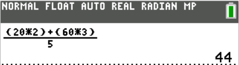
What was the associate's average daily commission for these 5 days?
$ A.\:\: \$40 \\[3ex] B.\:\: \$41 \\[3ex] C.\:\: \$44 \\[3ex] D.\:\: \$45 \\[3ex] E.\:\: \$46 \\[3ex] $
Average implies Arithmetic Mean
$20 on Monday and Tuesday (2 days)
$60 on Wednesday, Thursday, and Friday (3 days)
$ Average = \bar{x} = \dfrac{\Sigma x}{n} \\[5ex] = \dfrac{(20 \cdot 2) + (60 \cdot 3)}{5} \\[5ex] = \dfrac{40 + 180}{5} \\[5ex] = \dfrac{220}{5} \\[5ex] = \$44 $
One of the following values is the mean of the 4 recorded heights.
Which one?
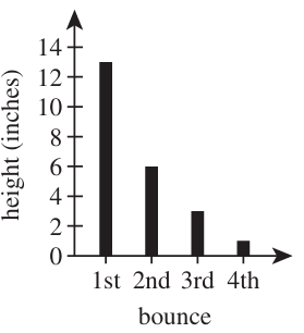
$ F.\;\; 2.30 \\[3ex] G.\;\; 2.50 \\[3ex] H.\;\; 4.50 \\[3ex] J.\;\; 5.75 \\[3ex] K.\;\; 7.00 \\[3ex] $
$ \text{Bounce} = 1st, 2nd, 3rd, 4th \\[3ex] \text{Data Values}, x = 13, 6, 3, 1 \\[3ex] \text{Sample size}, n = 4 \\[3ex] \bar{x} = \dfrac{\Sigma x}{n} \\[5ex] = \dfrac{13 + 6 + 3 + 1}{4} \\[5ex] = \dfrac{23}{4} \\[5ex] = 5.75 $
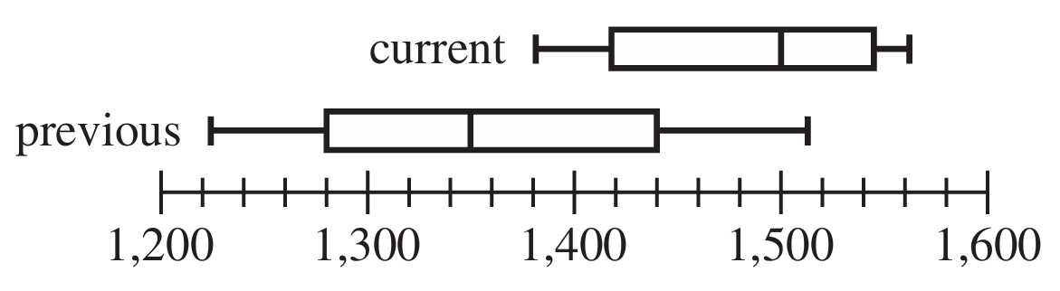
The table below gives the average daily attendance for each grade level at JFK High School for 4 months of the current school year.
The boxplots below show the distribution of JFK's total daily attendance figures for the previous school year (180 days) and for half of the current schoolyear (90 days).
| Month | ||||
| Grade | Sept. | Oct. | Nov. | Dec. |
|
9th 10th 11th 12th |
267 425 382 441 |
295 414 398 384 |
310 395 395 414 |
244 341 389 407 |
Only 18 students are taking none of the 3 courses.
The data are shown in the Venn diagram below.
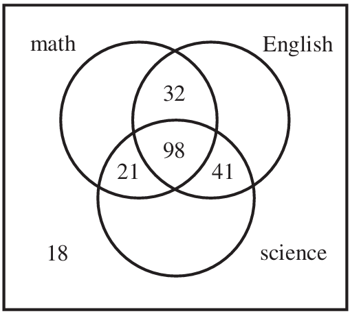
One of the juniors from Northeast High School will be chosen at random.
What is the probability that the chosen student is taking exactly 1 of these 3 courses?
$ A.\;\; 0.30 \\[3ex] B.\;\; 0.33 \\[3ex] C.\;\; 0.36 \\[3ex] D.\;\; 0.64 \\[3ex] E.\;\; 0.67 \\[3ex] $
The number of juniors taking exactly 1 of these 3 courses are those taking:
math only or
science only or
English only
This is: 300 − (32 + 41 + 21 + 98 + 18)
= 300 − 210
= 90
$ P(\text{taking exactly 1 of these 3 courses}) = \dfrac{n(\text{taking exactly 1 of these 3 courses})}{n(S)} \\[5ex] = \dfrac{90}{300} \\[5ex] = 0.3 $
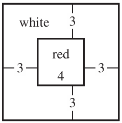
Each 4-inch-long side of the red square is parallel to 2 sides of the white square and is 3 inches from the closest side of the white square.
A dart will be thrown randomly and will land on the dartboard.
What is the probability that the dart will land on the red square?
$ A.\;\; \dfrac{1}{10} \\[5ex] B.\;\; \dfrac{1}{7} \\[5ex] C.\;\; \dfrac{2}{5} \\[5ex] D.\;\; \dfrac{4}{25} \\[5ex] E.\;\; \dfrac{16}{49} \\[5ex] $
$ \text{Area of Red Square} = 4^2 = 16\;\;square\;\;inches \\[4ex] \text{Area of Dartboard} = (3 + 4 + 3)^2 = 10^2 = 100\;\;square\;\;inches \\[4ex] P(Red\;\;Square) = \dfrac{\text{Area of Red Square}}{\text{Area of Dartboard}} \\[5ex] = \dfrac{16}{100} \\[5ex] = \dfrac{4}{25} $
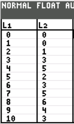
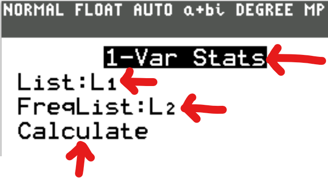
The frequency distribution of their scores is given below.
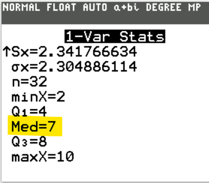
What was the median score for the class?
| Score | Frequency |
|---|---|
|
0 1 2 3 4 5 6 7 8 9 10 |
0 0 1 3 5 2 3 5 6 4 3 |
$ A.\;\; 3 \\[3ex] B.\;\; 5 \\[3ex] C.\;\; 6 \\[3ex] D.\;\; 7 \\[3ex] E.\;\; 8 \\[3ex] $
$ \Sigma F = 32 ...\text{class of 32 students} \\[3ex] \dfrac{\Sigma F}{2} = \dfrac{32}{2} = 16 \\[5ex] 0 + 0 = 0 + 1 = 1 + 3 = 4 + 5 = 9 + 2 = 11 + 3 = 14 + 5 = 19...STOP \\[3ex] 5\;\;\text{is the point of focus} \\[3ex] \text{What number has that frequency of }5? \\[3ex] Median = 7 $
Due to the time limit on the ACT, this calculator solution is not recommended.
However, if you know you can enter in data accurately and speedily (less than 30 seconds), you may go for it.
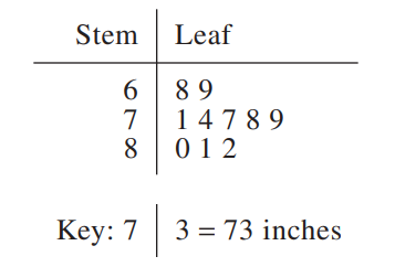
What is the probability that a long jump participant chosen at random from the competition will have jumped at least 75 inches?
$ A.\;\; \dfrac{3}{13} \\[5ex] B.\;\; \dfrac{7}{13} \\[5ex] C.\;\; \dfrac{3}{10} \\[5ex] D.\;\; \dfrac{4}{10} \\[5ex] E.\;\; \dfrac{6}{10} \\[5ex] $
$ n(S) = 10 \\[3ex] n(\ge 75) = 6 \\[3ex] P(\ge 75) = \dfrac{n(\ge 75)}{n(S)} = \dfrac{6}{10} $
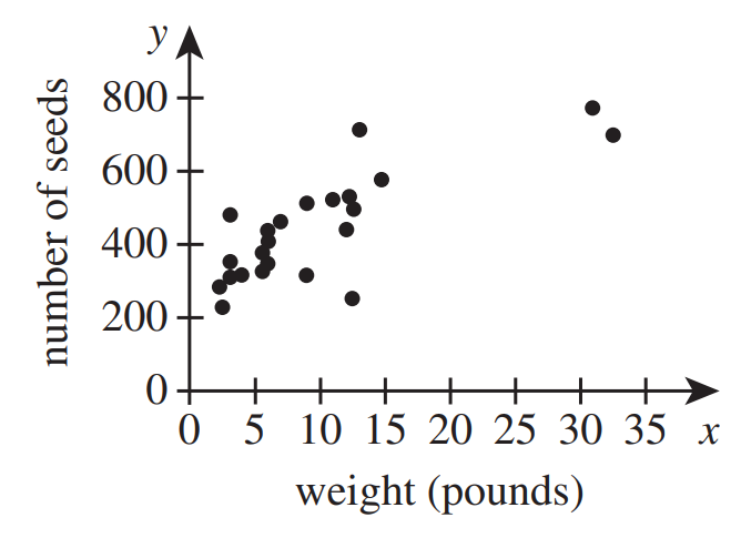
In a science class, students measured the weights, in pounds, of 23 pumpkins and counted the seeds in each pumpkin.
A scatterplot of the data is shown below.
To the nearest pound, the average weight of these pumpkins was 10 pounds, and the average number of seeds per pumpkin was 444 seeds.
An equation of the regression line of best fit is y = 15x + 294, where x is the weight, in pounds, and y is the number of seeds.
Each point has 2 integer coordinates.
The x-coordinate is the number of hours the student spent studying for a retake test, and the y-coordinate is the change in score from the original test to the retake test.
Noel drew the line shown through 2 data points to help predict future changes in score.
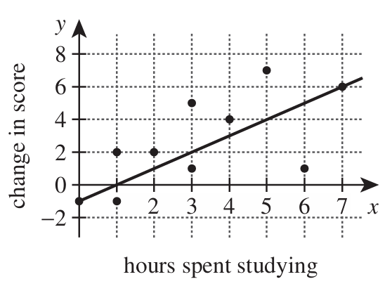
What is the median number of hours spent studying by all 10 students?
$ A.\;\; 2.0 \\[3ex] B.\;\; 2.5 \\[3ex] C.\;\; 3.0 \\[3ex] D.\;\; 3.2 \\[3ex] E.\;\; 3.5 \\[3ex] $
The middle numbers are in darkblue
The hours (in ascending order) are: 0, 1, 1, 2, 3, 3, 4, 5, 6, 7
$ Median = \dfrac{3 + 3}{2} \\[5ex] = \dfrac{6}{2} \\[5ex] = 3 $
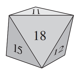
What is the probability that, on 1 toss of this octahedron, the number on the face landing down is a prime number or an even number?
$ A.\;\; 0 \\[3ex] B.\;\; \dfrac{1}{8} \\[5ex] C.\;\; \dfrac{1}{4} \\[5ex] D.\;\; \dfrac{1}{2} \\[5ex] E.\;\; \dfrac{7}{8} \\[5ex] $
Let:
the sample space = S
the set of prime numbers = R
the set of even numbers = E
probability = P
cardinality = n
$ S = \{1, 2, 3, 4, 5, 6, 7, 8\} \\[3ex] n(S) = 8 \\[5ex] R = \{2, 3, 5, 7\} \\[3ex] n(R) = 4 \\[5ex] E = \{2, 4, 6, 8\} \\[3ex] n(E) = 4 \\[5ex] R \cap E = \{2\} \\[3ex] n(R \cap E) = n(R \hspace{1em}AND\hspace{1em} E) = 1 \\[5ex] P(R \hspace{1em}OR\hspace{1em} E) \\[3ex] = \dfrac{n(R) + n(E) - n(R \hspace{1em}AND\hspace{1em} E)}{n(S)}...\text{Addition Law} \\[5ex] = \dfrac{4 + 4 - 1}{8} \\[5ex] = \dfrac{7}{8} $
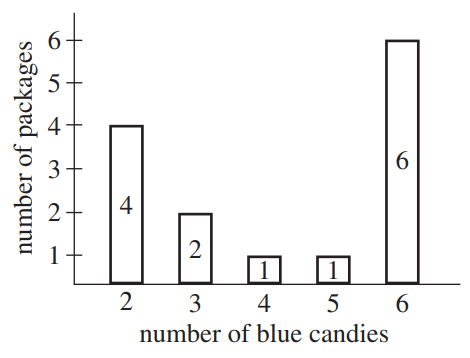
What is the median of the numbers of blue candies in the 14 packages?
$ A.\;\; 4.0 \\[3ex] B.\;\; 4.2 \\[3ex] C.\;\; 4.5 \\[3ex] D.\;\; 5.0 \\[3ex] E.\;\; 6.0 \\[3ex] $
Let us represent the bar graph in a table.
I think it is easier to work with tables.
| number of blue candies, x | number of packages, F |
|---|---|
| 2 | 4 |
| 3 | 2 |
| 4 | 1 |
| 5 | 1 |
| 6 | 6 |
$ \text{To find the median:} \\[3ex] \Sigma F = 14 \\[3ex] \dfrac{\Sigma F}{2} = \dfrac{14}{2} = 7 \\[5ex] \text{Begin from the top} \\[3ex] 4 + 2 = 6 \\[3ex] 6 + 1 = 7...STOP \\[3ex] x = 4 \\[5ex] \text{Begin from the bottom} \\[3ex] 6 + 1 = 7 ...STOP \\[3ex] x = 5 \\[5ex] Median = \dfrac{4 + 5}{2} \\[5ex] = \dfrac{9}{2} \\[5ex] = 4.5 $
The variables a − h represent 8 consecutive positive integers in order from least to greatest.
The frequencies of a, f, g, and h are equal; the frequency of e is 2 times the frequency of a; the frequency of b and of d is 3 times the frequency of a; and the frequency of c is 4 times the frequency of a.
Which of the following statements about the mean, median, and mode of the data set is true?
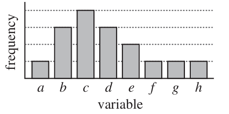
A. The mode is less than the median, and the median is less than the mean.
B. The mean is less than the median, and the median is less than the mode.
C. The mode is equal to the mean, and the mean id less than the median.
D. The mode is less than the mean, and the mean is equal to the median.
E. The mean is equal to the median, and the median is equal to the mode.
For a:
Left-skewed distribution (longer tail on the left): Mean < Median < Mode
Symmetric distribution: Mean = Median = Mode
Right-skewed distribution (longer tail on the right): Mean > Median > Mode
The distribution is right-skewed; hence the mean is greater than the median, and the median is greater than the mode.
This implies that:
The mode is less than the median, and the median is less than the mean.
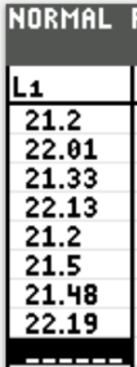
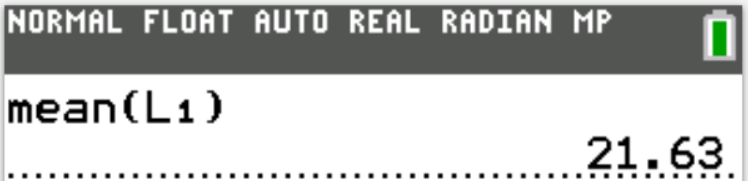
$ F.\;\; 21.20 \\[3ex] G.\;\; 21.27 \\[3ex] H.\;\; 21.49 \\[3ex] J.\;\; 21.63 \\[3ex] K.\;\; 22.07 \\[3ex] $
$ \Sigma Time = 21.2 + 22.01 + 21.33 + 22.13 + 21.2 + 21.5 + 21.48 + 22.19 = 173.04 \\[3ex] n = 8\;students \\[3ex] Mean, \bar{x} = \dfrac{\Sigma Time}{n} = \dfrac{173.04}{8} = 21.63 $
She plotted the data in the standard (x, y) coordinate plane below with the amount of the check on the x-axis and the amount of the tip on the y-axis.
Sumiko then performed a linear regression on the data, finding the regression equation to be $y = 0.16x − 0.44$ with a correlation coefficient, r, of 0.81.
She also graphed the regression line.
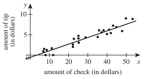
From her statistical analysis, Sumiko can correctly conclude that every $1 increase in the total amount of the check will result in approximately:
F. a 16 cent increase in her tip.
G. a 44 cent increase in her tip.
H. an 81 cent increase in her tip.
J. a 16 cent decrease in her tip.
K. a 44 cent decrease in her tip.
Regression Equation: $y = 0.16x − 0.44$
x = amount of check (in dollars)
y = amount of tip (in dollars)
Slope = $0.16 = 16 cents
This is a positive slope. The interpretation for the slope in this context implies that: On average, for every unit change ($1 increase in) in x (the amount of check), the y (amount of tip) increases by the slope (16 cents).
From her statistical analysis, Sumiko can correctly conclude that every $1 increase in the total amount of the check will result in approximately a 16 cent increase in her tip.


