Statistics and Probability
Welcome to Our Site
I greet you this day,
These are the solutions to the SACE past questions on Statistics and Probability.
The TI-84 Plus CE shall be used for applicable questions.
The link to the video solutions will be provided for you. Please subscribe to the YouTube channel to be notified
of upcoming livestreams.
You are welcome to ask questions during the video livestreams.
If you find these resources valuable and if any of these resources were helpful in your passing the
Mathematics papers of the SACE, please consider making a donation:
Cash App: $ExamsSuccess or
cash.app/ExamsSuccess
PayPal: @ExamsSuccess or
PayPal.me/ExamsSuccess
Google charges me for the hosting of this website and my other
educational websites. It does not host any of the websites for free.
Besides, I spend a lot of time to type the questions and the solutions well.
As you probably know, I provide clear explanations on the solutions.
Your donation is appreciated.
Comments, ideas, areas of improvement, questions, and constructive criticisms are welcome.
Feel free to contact me. Please be positive in your message.
I wish you the best.
Thank you.
-
Symbols and Meanings
- $X$ = dataset $X$
- $x = x-values$ OR data values
- $x_{mid}$ = class midpoint of $x-values$ = class midpoint of the data values
- $\Sigma$ (pronounced as uppercase Sigma) = $summation$
- $\Sigma x$ = summation of the $x-values$
- $f = frequency$
- $F = frequency$
- $\Sigma f$ = summation of the frequencies
- $\Sigma fx$ = summation of the product of the $x-values$ and their corresponding frequencies
- $(\Sigma x)^2$ = square of the summation of the $x-values$
- $\Sigma x^2$ = summation of the squared of the $x-values$
- $\bar{x}$ is sample mean of the $x-values$
- $\mu$ = population mean
- $n$ = sample size
- $N$ = population size
- $\tilde{x}$ = median
- $\widehat{x}$ = mode
- $AM$ = assumed mean
- $D$ = deviation from the assumed mean
- $x_{MR}$ = midrange
- $LCL$ = lower class limit
- $UCL$ = upper class limit
- $min$ = minimum data value
- $max$ = maximum data value
- $LCB_{med}$ = lower class boundary of the median class
- $CW$ = class width
- $f_{med}$ = frequency of the median class
- $CF_{bmed}$ = cumulative frequency of the class before the median class
- $LCB_{mod}$ = lower class boundary of the modal class
- $f_{mod}$ = frequency of the modal class
- $f_{bmod}$ = frequency of the class before the modal class
- $f_{amod}$ = frequency of the class after the modal class
- $R$ = range
- $s$ = sample standard deviation
- $s^2$ = sample variance
- $\sigma$ = population standard deviation
- $\sigma^2$ = population variance
- $CV$ = coefficient of variation
- $z = z-score$
- $Q_1$ = lower quartile or first quartile
- $P_{25}$ = 25th percentile or first quartile
- $Q_2$ = middle quartile or second quartile or median
- $P_{50}$ = 50th percentile or median
- $Q_3$ = upper quartile or third quartile
- $P_{75}$ = 75th percentile or third quartile
- $IQR$ = interquartile range
- $SIQR$ = semi-interquartile range
- $MQ$ = midquartile
- $LF$ = lower fence
- $UF$ = upper fence
- $TM$ = trimmed mean
- $\Pi$ (pronounced as uppercase Pi) = $product$
- $\Pi x$ = product of the $x-values$
- $GM$ = geometric mean
Grouped Data
$
\underline{\text{Class Size or Class Width}} \\[3ex]
(1.)\;\; Class\:\:Width = \dfrac{Maximum - Minimum}{Number\:\:of\:\:classes} \\[5ex]
(2.)\;\; Class\:\:Width = LCI\:\:of\:\:2nd\:\:Class - LCI\:\:of\:\:1st\:\:Class \\[3ex]
(3.)\;\; Class\:\:Width = UCI\:\:of\:\:2nd\:\:Class - UCI\:\:of\:\:1st\:\:Class \\[3ex]
(4.)\;\; Class\:\:Width = UCB\:\:of\:\:a\:\:class - LCB\:\:of\:\:the\:\:same\:\:class \\[3ex]
(5.)\;\; Class\:\:Width = LCB\:\:of\:\:a\:\:Class - LCB\:\:of\:\:previous\:\:class \\[5ex]
\underline{\text{Frequency Density}} \\[3ex]
(6.)\;\; \text{Frequency Density} = \dfrac{\text{Frequency}}{\text{Class Width}} \\[7ex]
\underline{\text{Class Midpoints or Class Marks}} \\[3ex]
(7.)\;\; Class\:\:Width = LCB\:\:of\:\:a\:\:Class - LCB\:\:of\:\:previous\:\:class \\[5ex]
\underline{\text{Class Boundaries}} \\[3ex]
(8.)\;\; Lower\:\:Class\:\:Boundary\:\:of\:\:a\:\:class = \dfrac{LCI\:\:of\:\:that\:\:class +
UCI\:\:of\:\:previous/preceding\:\:class}{2} \\[5ex]
(9.)\;\; Upper\:\:Class\:\:Boundary\:\:of\:\:a\:\:class = \dfrac{UCI\:\:of\:\:that\:\:class +
LCI\:\:of\:\:next/succeeding\:\:class}{2} \\[5ex]
$
(10.) Shortcut for Class Boundaries
If the class intervals are integers:
Lower Class Boundary = Lower Class Interval − 0.5
Upper Class Boundary = Upper Class Interval + 0.5
If the class intervals are decimals in one decimal place:
Lower Class Boundary = Lower Class Interval − 0.05
Upper Class Boundary = Upper Class Interval + 0.05
If the class intervals are decimals in two decimal places:
Lower Class Boundary = Lower Class Interval − 0.005
Upper Class Boundary = Upper Class Interval + 0.005
...and so on and so forth.
$
\underline{\text{Relative Frequency}} \\[3ex]
(11.)\;\; RF\:\:of\:\:a\:\:class = \dfrac{Frequency\:\:of\:\:that\:\:class}{\Sigma Frequency} \\[7ex]
\underline{\text{Cumulative Frequency}} \\[3ex]
(12.)\;\; CF\:\:of\:\:1st\:\:Class = Frequency\:\:of\:\:1st\:\:Class \\[3ex]
CF\:\:of\:\:2nd\:\:Class = Frequency\:\:of\:\:1st\:\:Class + Frequency\:\:of\:\:2nd\:\:Class \\[3ex]
CF\:\:of\:\:3rd\:\:Class = Frequency\:\:of\:\:1st\:\:Class + Frequency\:\:of\:\:2nd\:\:Class +
Frequency\:\:of\:\:3rd\:\:Class \\[3ex]
CF = CF\:\:of\:\:Last\:\:Class = \Sigma Frequency
$
Measures of Center: Raw Data and Ungrouped Data
$ \underline{Sample\:\:Mean} \\[3ex] (1.)\:\: \bar{x} = \dfrac{\Sigma x}{n} \\[5ex] (2.)\:\: n = \Sigma f \\[3ex] (3.)\:\: \bar{x} = \dfrac{\Sigma fx}{\Sigma f} \\[5ex] \underline{Given\:\:an\:\:Assumed\:\:Mean} \\[3ex] (4.)\:\: D = x - AM \\[3ex] (5.)\:\: \bar{x} = AM + \dfrac{\Sigma D}{n} \\[5ex] (6.)\:\: \bar{x} = AM + \dfrac{\Sigma fD}{\Sigma f} \\[7ex] \underline{Population\:\:Mean} \\[3ex] (7.)\:\: \mu = \dfrac{\Sigma x}{N} \\[5ex] (8.)\:\: N = \Sigma f \\[3ex] \underline{Given\:\:an\:\:Assumed\:\:Mean} \\[3ex] (9.)\:\: D = x - AM \\[3ex] (10.)\:\: \mu = AM + \dfrac{\Sigma D}{N} \\[5ex] (11.)\:\: \mu = AM + \dfrac{\Sigma fD}{\Sigma f} \\[7ex] \underline{Median} \\[3ex] (12.)\:\: \tilde{x} = \left(\dfrac{\Sigma f + 1}{2}\right)th \:\:for\:\:sorted\:\:odd\:\:sample\:\:size \\[5ex] (13.)\:\: \tilde{x} = \left(\dfrac{\Sigma f}{2}\right)th \:\:for\:\:sorted\:\:even\:\:sample\:\:size \\[7ex] \underline{Mode} \\[3ex] (14.)\:\: Mode = x-value(s) \:\;with\:\:highest\:\:frequency \\[5ex] \underline{Midrange} \\[3ex] (15.)\:\: x_{MR} = \dfrac{min + max}{2} \\[5ex] \underline{Geometric\;\;Mean} \\[3ex] (16.)\;\; GM = \sqrt[n]{\prod\limits_{x=1}^n x} $
Measures of Center: Grouped Data
$ \underline{Class\:\:Midpoint} \\[3ex] (1.)\:\: x_{mid} = \dfrac{LCL + UCL}{2} \\[7ex] Equal\:\:Class\:\:Intervals\:(Same\:\:Class\:\:Size) \\[3ex] \underline{Mean} \\[3ex] (2.)\:\: \bar{x} = \dfrac{\Sigma fx_{mid}}{\Sigma f} \\[7ex] Equal\:\:Class\:\:Intervals\:(Same\:\:Class\:\:Size) \\[3ex] \underline{Given\:\:an\:\:Assumed\:\:Mean} \\[3ex] (3.)\:\: D = x_{mid} - AM \\[3ex] (4.)\:\: \bar{x} = AM + \dfrac{\Sigma fD}{\Sigma f} \\[7ex] \underline{Median} \\[3ex] (5.)\:\: \tilde{x} = LCB_{med} + \dfrac{CW}{f_{med}} * \left[\left(\dfrac{\Sigma f}{2}\right) - CF_{bmed}\right] \\[7ex] \underline{Mode} \\[3ex] (6.)\:\: \widehat{x} = LCB_{mod} + CW * \left[\dfrac{f_{mod} - f_{bmod}}{(f_{mod} - f_{bmod}) + (f_{mod} - f_{amod})}\right] $
Measures of Spread: Raw Data and Ungrouped Data
$ \underline{Range} \\[3ex] (1.)\:\: Range = max - min \\[3ex] \underline{Using\;\;Assumed\;\;Mean} \\[3ex] (2.)\;\; D = x - AM \\[5ex] \underline{Sample\:\:Variance} \\[3ex] \color{red}{First\:\:Formula} \\[3ex] (3.)\:\: s^2 = \dfrac{\Sigma(x - \bar{x})^2}{n - 1} \\[5ex] (4.)\:\: s^2 = \dfrac{\Sigma f(x - \bar{x})^2}{\Sigma f - 1} \\[5ex] \color{red}{Second\:\:Formula} \\[3ex] (5.)\:\: s^2 = \dfrac{n(\Sigma x^2) - (\Sigma x)^2}{n(n - 1)} \\[5ex] (6.)\:\: s^2 = \dfrac{\Sigma f(\Sigma fx^2) - (\Sigma fx)^2}{\Sigma f(\Sigma f - 1)} \\[7ex] \underline{Using\;\;Assumed\;\;Mean} \\[3ex] (7.)\;\; s^2 = \dfrac{\Sigma D^2}{n - 1} - \left(\dfrac{\Sigma D}{n - 1}\right)^2 \\[7ex] (8.)\;\; s^2 = \dfrac{\Sigma fD^2}{\Sigma f - 1} - \left(\dfrac{\Sigma fD}{\Sigma f - 1}\right)^2 \\[10ex] \underline{Population\:\:Variance} \\[3ex] \color{red}{First\:\:Formula} \\[3ex] (9.)\:\: \sigma^2 = \dfrac{\Sigma(x - \mu)^2}{N} \\[5ex] (10.)\:\: \sigma^2 = \dfrac{\Sigma f(x - \mu)^2}{\Sigma f} \\[5ex] \color{red}{Second\:\:Formula} \\[3ex] (11.)\:\: \sigma^2 = \dfrac{N(\Sigma x^2) - (\Sigma x)^2}{N^2} \\[5ex] (12.)\:\: \sigma^2 = \dfrac{\Sigma f(\Sigma fx^2) - (\Sigma fx)^2}{(\Sigma f)^2} \\[7ex] \underline{Using\;\;Assumed\;\;Mean} \\[3ex] (13.)\;\; \sigma^2 = \dfrac{\Sigma D^2}{N} - \left(\dfrac{\Sigma D}{N}\right)^2 \\[7ex] (14.)\;\; \sigma^2 = \dfrac{\Sigma fD^2}{\Sigma f} - \left(\dfrac{\Sigma fD}{\Sigma f}\right)^2 \\[10ex] \underline{Sample\:\:Standard\:\:Deviation} \\[3ex] \color{red}{First\:\:Formula} \\[3ex] (15.)\:\: s = \sqrt{\dfrac{\Sigma(x - \bar{x})^2}{n - 1}} \\[5ex] (16.)\:\: s = \sqrt{\dfrac{\Sigma f(x - \bar{x})^2}{\Sigma f - 1}} \\[5ex] \color{red}{Second\:\:Formula} \\[3ex] (17.)\:\: s = \sqrt{\dfrac{n(\Sigma x^2) - (\Sigma x)^2}{n(n - 1)}} \\[5ex] (18.)\:\: s = \sqrt{\dfrac{\Sigma f(\Sigma fx^2) - (\Sigma fx)^2}{\Sigma f(\Sigma f - 1)}} \\[7ex] \underline{Using\;\;Assumed\;\;Mean} \\[3ex] (19.)\;\; s = \sqrt{\dfrac{\Sigma D^2}{n - 1} - \left(\dfrac{\Sigma D}{n - 1}\right)^2} \\[7ex] (20.)\;\; s = \sqrt{\dfrac{\Sigma fD^2}{\Sigma f - 1} - \left(\dfrac{\Sigma fD}{\Sigma f - 1}\right)^2} \\[10ex] \underline{Population\:\:Standard\:\:Deviation} \\[3ex] \color{red}{First\:\:Formula} \\[3ex] (21.)\:\: \sigma = \sqrt{\dfrac{\Sigma(x - \mu)^2}{N}} \\[5ex] (22.)\:\: \sigma = \sqrt{\dfrac{\Sigma f(x - \mu)^2}{\Sigma f}} \\[5ex] \color{red}{Second\:\:Formula} \\[3ex] (23.)\:\: \sigma = \dfrac{\sqrt{N(\Sigma x^2) - (\Sigma x)^2}}{N} \\[5ex] (24.)\:\: \sigma = \dfrac{\sqrt{\Sigma f(\Sigma fx^2) - (\Sigma fx)^2}}{\Sigma f} \\[7ex] \underline{Using\;\;Assumed\;\;Mean} \\[3ex] (25.)\;\; \sigma = \sqrt{\dfrac{\Sigma D^2}{N} - \left(\dfrac{\Sigma D}{N}\right)^2} \\[7ex] (26.)\;\; \sigma = \sqrt{\dfrac{\Sigma fD^2}{\Sigma f} - \left(\dfrac{\Sigma fD}{\Sigma f}\right)^2} \\[10ex] \underline{Range\:\:Rule\:\:of\:\:Thumb} \\[3ex] Approximate\:\:Value\:\:of\:\:Calculating\:\:Standard\:\:Deviation \\[3ex] (27.)\:\: s = \dfrac{Range}{4} = \dfrac{max - min}{4} \\[7ex] \underline{Interquartile\:\:Range} \\[3ex] (28.)\:\: IQR = Q_3 - Q_1 \\[5ex] \underline{Coefficient\:\:of\:\:Variation\:\:for\:\:Sample} \\[3ex] (29.)\:\: CV = \dfrac{s}{x} * 100 ...in\:\:\% \\[7ex] \underline{Coefficient\:\:of\:\:Variation\:\:for\:\:Population} \\[3ex] (30.)\:\: CV = \dfrac{\sigma}{x} * 100 ...in\:\:\% \\[7ex] \underline{Mean\:\:Absolute\:\:Deviation} \\[3ex] (31.)\:\: MAD = \dfrac{\Sigma |x - \bar{x}|}{n} \\[5ex] \underline{Mean\:\:Absolute\:\:Deviation} \\[3ex] (32.)\:\: MAD = \dfrac{\Sigma f|x - \bar{x}|}{\Sigma f} \\[5ex] $
Measures of Spread: Grouped Data
$ \underline{Class\:\:Midpoint} \\[3ex] (1.)\:\: x_{mid} = \dfrac{LCL + UCL}{2} \\[5ex] \underline{Using\;\;Assumed\;\;Mean} \\[3ex] (2.)\;\; D = x_{mid} - AM \\[5ex] \underline{Sample\:\:Variance} \\[3ex] \color{red}{First\:\:Formula} \\[3ex] (3.)\:\: s^2 = \dfrac{\Sigma f(x_{mid} - \bar{x})^2}{\Sigma f - 1} \\[5ex] \color{red}{Second\:\:Formula} \\[3ex] (4.)\:\: s^2 = \dfrac{\Sigma f(\Sigma fx_{mid}^2) - (\Sigma fx_{mid})^2}{\Sigma f(\Sigma f - 1)} \\[5ex] \underline{Using\;\;Assumed\;\;Mean} \\[3ex] (5.)\;\; s^2 = \dfrac{\Sigma D^2}{n - 1} - \left(\dfrac{\Sigma D}{n - 1}\right)^2 \\[7ex] (6.)\;\; s^2 = \dfrac{\Sigma fD^2}{\Sigma f - 1} - \left(\dfrac{\Sigma fD}{\Sigma f - 1}\right)^2 \\[10ex] \underline{Sample\:\:Standard\:\:Deviation} \\[3ex] \color{red}{First\:\:Formula} \\[3ex] (7.)\:\: s = \sqrt{\dfrac{\Sigma f(x_{mid} - \bar{x})^2}{\Sigma f - 1}} \\[5ex] \color{red}{Second\:\:Formula} \\[3ex] (8.)\:\: s = \sqrt{\dfrac{\Sigma f(\Sigma fx_{mid}^2) - (\Sigma fx_{mid})^2}{\Sigma f(\Sigma f - 1)}} \\[5ex] \underline{Using\;\;Assumed\;\;Mean} \\[3ex] (9.)\;\; s = \sqrt{\dfrac{\Sigma D^2}{n} - \left(\dfrac{\Sigma D}{n - 1}\right)^2} \\[7ex] (10.)\;\; s = \sqrt{\dfrac{\Sigma fD^2}{\Sigma f - 1} - \left(\dfrac{\Sigma fD}{\Sigma f - 1}\right)^2} \\[10ex] \underline{Population\:\:Variance} \\[3ex] \color{red}{First\:\:Formula} \\[3ex] (11.)\:\: \sigma^2 = \dfrac{\Sigma f(x_{mid} - \bar{x})^2}{\Sigma f} \\[5ex] \color{red}{Second\:\:Formula} \\[3ex] (12.)\:\: \sigma^2 = \dfrac{\Sigma f(\Sigma fx_{mid}^2) - (\Sigma fx_{mid})^2}{\Sigma f(\Sigma f)} \\[5ex] \underline{Using\;\;Assumed\;\;Mean} \\[3ex] (13.)\;\; \sigma^2 = \dfrac{\Sigma D^2}{N} - \left(\dfrac{\Sigma D}{N}\right)^2 \\[7ex] (14.)\;\; \sigma^2 = \dfrac{\Sigma fD^2}{\Sigma f} - \left(\dfrac{\Sigma fD}{\Sigma f}\right)^2 \\[10ex] \underline{Population\:\:Standard\:\:Deviation} \\[3ex] \color{red}{First\:\:Formula} \\[3ex] (15.)\:\: \sigma = \sqrt{\dfrac{\Sigma f(x_{mid} - \bar{x})^2}{\Sigma f}} \\[5ex] \color{red}{Second\:\:Formula} \\[3ex] (16.)\:\: \sigma = \sqrt{\dfrac{\Sigma f(\Sigma fx_{mid}^2) - (\Sigma fx_{mid})^2}{\Sigma f(\Sigma f)}} \\[5ex] \underline{Using\;\;Assumed\;\;Mean} \\[3ex] (17.)\;\; \sigma = \sqrt{\dfrac{\Sigma D^2}{N} - \left(\dfrac{\Sigma D}{N}\right)^2} \\[7ex] (18.)\;\; \sigma = \sqrt{\dfrac{\Sigma fD^2}{\Sigma f} - \left(\dfrac{\Sigma fD}{\Sigma f}\right)^2} \\[10ex] $
Measures of Position
A data value is usual if $-2.00 \le z-score \le 2.00$
A data value is unusual if $z-score \lt -2.00$ OR $z-score \gt 2.00$
$
\underline{Sample} \\[3ex]
Minimum\:\:usual\:\:data\:\:value = \bar{x} - 2s \\[3ex]
Maximum\:\:usual\:\:data\:\:value = \bar{x} + 2s \\[5ex]
\underline{Population} \\[3ex]
Minimum\:\:usual\:\:data\:\:value = \mu - 2\sigma \\[3ex]
Maximum\:\:usual\:\:data\:\:value = \mu + 2\sigma \\[5ex]
\underline{z\:\:score\:\:for\:\:Sample} \\[3ex]
(1.)\:\: z = \dfrac{x - \bar{x}}{s} \\[7ex]
\underline{z\:\:score\:\:for\:\:Population} \\[3ex]
(2.)\:\: z = \dfrac{x - \mu}{\sigma} \\[7ex]
\underline{Quantiles(Percentiles,\:Deciles,\:Quintiles,\:and\:Quartiles)} \\[3ex]
\color{red}{Convert\:\:a\:\:Data\:\:value\:\:to\:\:a\:\:Quantile} \\[3ex]
x\:\:and\:\:y\:\:are\:\:two\:\:different\:\:variables \\[3ex]
(3.)\:\: Percentile\:\:of\:\:x =
\dfrac{number\:\:of\:\:values\:\:less\:\:than\:\:x}{total\:\:number\:\:of\:\:values} * 100 = yth\:\:Percentile
\\[5ex]
(4.)\:\: Decile\:\:of\:\:x =
\dfrac{number\:\:of\:\:values\:\:less\:\:than\:\:x}{total\:\:number\:\:of\:\:values} * 10 = yth\:\:Decile
\\[5ex]
(5.)\:\: Quintile\:\:of\:\:x =
\dfrac{number\:\:of\:\:values\:\:less\:\:than\:\:x}{total\:\:number\:\:of\:\:values} * 5 = yth\:\:Quintile
\\[5ex]
(6.)\:\: Quartile\:\:of\:\:x =
\dfrac{number\:\:of\:\:values\:\:less\:\:than\:\:x}{total\:\:number\:\:of\:\:values} * 4 = yth\:\:Quartile
\\[7ex]
\color{red}{Convert\:\:a\:\:Quantile\:\:to\:\:a\:\:Data\:\:Value} \\[3ex]
Calculate\:\:the\:\:xth\:\:position\:\:of\:\:the\:\:yth\:\:Quantile \\[3ex]
(7.)\:\: xth\:\:position = \dfrac{yth\:\:Percentile}{100} * total\:\:number\:\:of\:\:values \\[5ex]
(8.)\:\: xth\:\:position = \dfrac{yth\:\:Decile}{10} * total\:\:number\:\:of\:\:values \\[5ex]
(9.)\:\: xth\:\:position = \dfrac{yth\:\:Quintile}{5} * total\:\:number\:\:of\:\:values \\[5ex]
(10.)\:\: xth\:\:position = \dfrac{yth\:\:Quartile}{4} * total\:\:number\:\:of\:\:values \\[7ex]
$
| If the $xth$ position | then, |
|---|---|
| is an integer |
$xth\:\:position = \dfrac{xth\:\:position + (x + 1)th\:\;position}{2}$ In other words, find the value of the $xth$ position; find the value of the next position; and determine the mean of the two values. |
| is not an integer | $xth$ position is rounded up |
$ \underline{The\:\:Five-Number\:\:Summary\:\:of\:\:Data} \\[3ex] (11.)\:\: Minimum\:(min) \\[3ex] (12.)\:\: Lower\:\:Quartile\:(Q_1) \\[3ex] (13.)\:\: Median\:\:or\:\:Middle\:\:Quartile\:(Q_2) \\[3ex] (14.)\:\: Upper\:\:Quartile\:(Q_3) \\[3ex] (15.)\:\: Maximum\:(Max) \\[5ex] \underline{Other\:\:Statistics\:\:from\:\:Quantiles} \\[3ex] (16.)\:\: IQR = Q_3 - Q_1 \\[3ex] (17.)\:\: SIQR = \dfrac{IQR}{2} = \dfrac{Q_3 - Q_1}{2} \\[5ex] (18.)\:\: MQ = \dfrac{Q_3 + Q_1}{2} \\[5ex] (19.)\:\: Upper\:\:Quartile\:(Q_3) \\[3ex] (20.)\:\: LF = Q_1 - 1.5(IQR) \\[3ex] (21.)\:\: UF = Q_3 + 1.5(IQR) $
Probability
Given any two events say A and B
$
P(E) = \dfrac{n(E)}{n(S)} \\[5ex]
\underline{\text{Addition Rule}} \\[3ex]
\dfrac{n(A \cup B)}{n(S)} = \dfrac{n(A)}{n(S)} + \dfrac{n(B)}{n(S)} - \dfrac{n(A \cap B)}{n(S)} \\[5ex]
P(A \cup B) = P(A) + P(B) - P(A \cap B) \\[3ex]
P(A\:\:\:OR\:\:\:B) = P(A) + P(B) - P(A\:\:\:AND\:\:\:B) \\[5ex]
$
For Independent Events
$
P(B|A) = P(B) \\[3ex]
\rightarrow P(A\:\:\:OR\:\:\:B) = P(A) + P(B) - [P(A) * P(B)] \\[5ex]
$
For Dependent Events
$
P(B|A) = P(B|A) \\[3ex]
\rightarrow P(A\:\:\:OR\:\:\:B) = P(A) + P(B) - [P(A) * P(B|A)] \\[5ex]
$
For Mutually Exclusive Events (Disjoint Events)
$
P(A \cap B) = 0 \\[3ex]
P(A\:\:\:OR\:\:\:B) = P(A) + P(B) - 0 \\[3ex]
\rightarrow P(A\:\:\:OR\:\:\:B) = P(A) + P(B) \\[5ex]
$
$
\underline{\text{Multiplication Rule}} \\[3ex]
P(A\:\:\:AND\:\:\:B) = P(A) * P(B|A) \\[3ex]
P(A \cap B) = P(A) * P(B|A) \\[3ex]
P(A\:\:\:AND\:\:\:B) = P(A \cap B) \\[5ex]
$
$P(B|A)$ is read as: the probability of event $B$ given event $A$
For Independent Events
$
P(B|A) = P(B) \\[3ex]
\rightarrow P(A\:\:\:AND\:\:\:B) = P(A) * P(B) \\[5ex]
$
For Dependent Events
$
P(B|A) = P(B|A) \\[3ex]
\rightarrow P(A\:\:\:AND\:\:\:B) = P(A) * P(B|A) \\[5ex]
$
The complement of Event $A$ is $A'$
$
\underline{Complementary\;\;Rule} \\[3ex]
P(A) + P(A') = 1 \\[3ex]
\rightarrow P(A') = 1 - P(A) \\[5ex]
$
Other Formulas
$
(1.)\;\; P(A) = P(A \cap B') + P(A \cap B)
$
Probability Distributions
$
\boldsymbol{Probability\;\;Distribution} \\[3ex]
(1.)\;\;\mu = \Sigma[x * P(x)] \\[3ex]
(2.)\;\;E = \Sigma[x * P(x)] \\[3ex]
(3.)\;\; \sigma = \sqrt{\Sigma[x^2 * P(x)] - \mu^2} \\[7ex]
\boldsymbol{Combinatorics} \\[3ex]
(1.)\:\: 0! = 1 \\[3ex]
(2.)\:\: n! = n * (n - 1) * (n - 2) * (n - 3) * ... * 1 \\[3ex]
(3.)\;\; n! = n * (n - 1)! \\[3ex]
(4.)\;\; n! = (n - 1) * (n - 2)!...among\;\;others \\[3ex]
(5.)\:\: C(n, x) = \dfrac{n!}{(n - x)!x!} \\[5ex]
(6.)\;\; C(n, x) = C(n, n - x) \\[7ex]
\boldsymbol{Binomial\;\;Distribution} \\[3ex]
(1.)\;\; p + q = 1 \\[3ex]
(2.)\;\; \mu = n * p \\[3ex]
(3.)\;\; \sigma = \sqrt{n * p * q} \\[4ex]
(4.)\;\; P(x) = C(n, x) * p^x * q^{n - x}...\text{Depends on the context of the question} \\[5ex]
where \\[3ex]
x = \text{number of successes/failures} \\[3ex]
n = \text{number of trials} = 12 \\[3ex]
C(n, x) = \text{Binomial coefficient} \\[3ex]
P(x) = \text{Probability of the number of successes/failures} \\[3ex]
p = \text{probability of success} = 70\% = 0.7 \\[3ex]
q = \text{probability of failure} = 1 - 0.7 = 0.3 \\[5ex]
\boldsymbol{Poisson\;\;Distribution} \\[3ex]
(1.)\;\;P(x) = \dfrac{\mu^x * e^{-\mu}}{x!} \\[5ex]
(2.)\;\; \mu = \sigma^2 \\[7ex]
\boldsymbol{Normal\;\;Distribution} \\[3ex]
(1.)\;\; z = \dfrac{x - \bar{x}}{s} \\[5ex]
(2.)\;\; x = \bar{x} + zs \\[3ex]
(3.)\;\; z = \dfrac{x - \mu}{\sigma} \\[5ex]
(4.)\;\; x = \mu + z\sigma \\[3ex]
(5.)\;\;\text{Probability Density Function},\;\;P(x) =
\dfrac{1}{\sigma\sqrt{2\pi}}e^{{-\dfrac{1}{2}}\left(\dfrac{x - \mu}{\sigma}\right)^2} \\[7ex]
$
Empirical Rule (68 - 95 - 99.7 percent Rule)
(Applies only to Normal Distribution)
(a.) 68% of the data lie within (below and above) 1 standard deviation of the mean
(b.) 95% of the data lie within (below and above) 2 standard deviations of the mean
(c.) 99.7% of the data lie within (below and above) 3 standard deviations of the mean
Pafnuty Chebyshev's Theorem
(Applies to any distribution)
At least $\left(1 - \dfrac{1}{k^2}\right) * 100$ % of the data lie within $k$ standard deviations of the mean
implies
At least $\left(1 - \dfrac{1}{k^2}\right) * 100$ % of the data lie within $\mu - k\sigma$ and $\mu + k\sigma$
Range Rule of Thumb
Minimum Usual Value = μ - 2σ
Maximum Usual Value = μ + 2σ
A data value is unusual if it is less than the minimum usual value or greater than the
maximum usual value
z-score Boundary
A data value is usual if −2.00 ≤ z-score ≤ 2.00
A data value is unusual if z-score < −2.00 or if z-score > 2.00
Specialist Mathematics Formula Sheet
(a.) Determine
(i.) Pr(50 ≤ X ≤ 52)
(ii.) Pr(X ≥ 58)
(b.) Given that Pr(X ≥ k) = 0.10, determine the value of k.
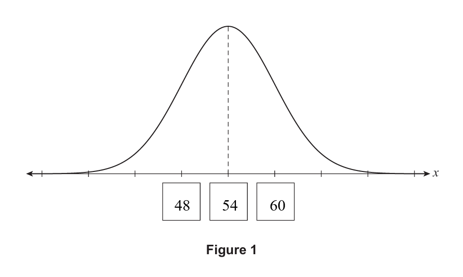
Figure 1 shows the graph of the probability density function for the random variable X.
The dashes on the x-axis show increments of one standard deviation.
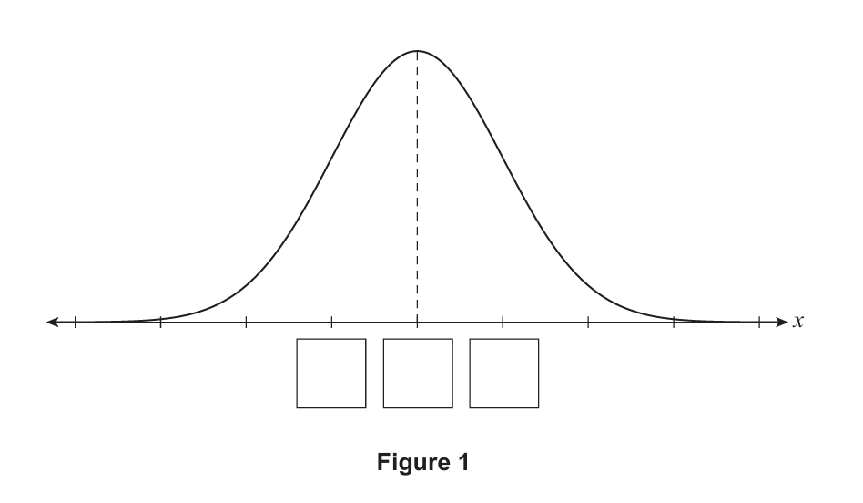
(c.) On Figure 1, write a number in each box to provide a scale for the x-axis.
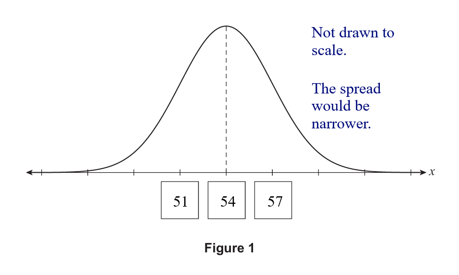
(d.) Let $\overline{X_4}$ be the random variable representing the sample mean of 4 independent observations of X.
(i.) State the mean and standard deviation of $\overline{X_4}$.
(ii.) On Figure 1 above, sketch the probability density function for the random variable $\overline{X_4}$.
(a.)
(i.)
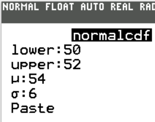
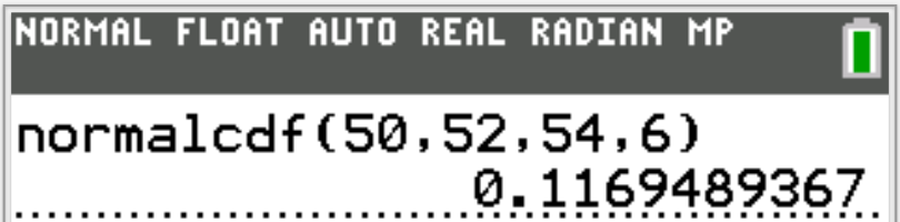
$ Pr(50 \le X \le 52) = 0.1169489367 \\[3ex] $ (ii.)
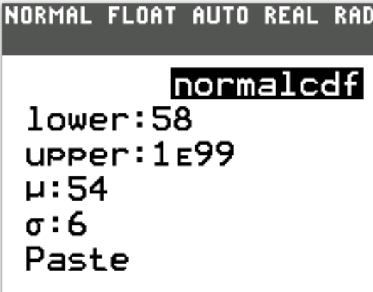
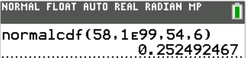
$ Pr(X \ge 58) = 0.252492467 \\[3ex] $ (b.)
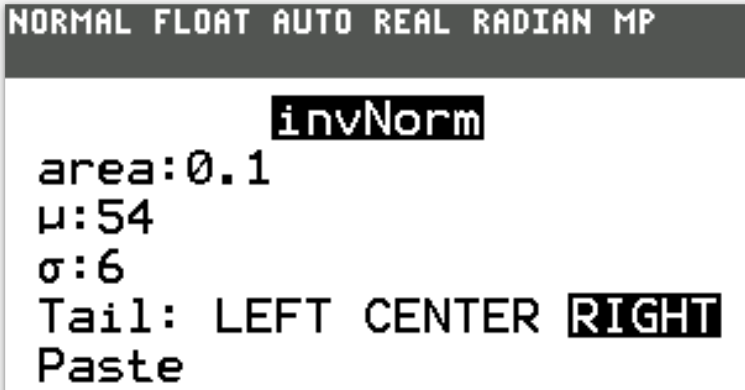
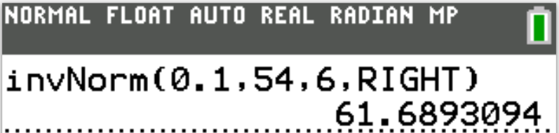
$ Pr(X \ge k) = 0.1 \\[3ex] k = 61.6893094 \\[5ex] (c.) \\[3ex] \mu - 1\sigma = 54 - 6 = 48 \\[3ex] \mu + 1\sigma = 54 + 6 = 60 \\[3ex] $ The number in each box is:
(d.) Let the:
Sample mean of 4 independent observations of X = $\overline{X_4}$
Mean of the sample mean of 4 independent observations of X (Mean of $\overline{X_4}$) = $\mu_{\overline{X_4}}$
Standard deviation of the sample mean of 4 independent observations of X (Standard deviation of $\overline{X_4}$) = $\sigma_{\overline{X_4}}$
Population mean = $\mu$
Population standard deviation = $\sigma$
$ (i.) \\[3ex] \underline{\text{Central Limit Theorem}} \\[3ex] n = 4 \\[3ex] \mu_{\overline{X_4}} = \mu \\[5ex] \sigma_{\overline{X_4}} \\[3ex] = \dfrac{\sigma}{\sqrt{n}} \\[5ex] = \dfrac{\sigma}{\sqrt{4}} \\[5ex] = \dfrac{\sigma}{2} \\[5ex] For: \\[3ex] \mu = 54 \\[3ex] \sigma = 6 \\[3ex] \mu_{\overline{X_4}} = 54 \\[3ex] \sigma_{\overline{X_4}} = \dfrac{6}{2} = 3 \\[3ex] \mu - 1\sigma = 54 - 3 = 51 \\[3ex] \mu + 1\sigma = 54 + 3 = 57 \\[3ex] $ (ii.) The sketch of the probability density function for the random variable $\overline{X_4}$ is: